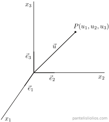
Index notation for tensors and vectors

Index notation is used extensively in the literature on stresses, strains and constitutive equations, because it drastically reduces the number of terms in an equation and simplifies the expressions. We will use a right-handed Cartesian coordinate system to describe index notation (cf. Fig. 1). It is also more convenient to name the axes $x_{1}$, $x_{2}$ and $x_{3}$ instead of the more familiar $x$, $y$ and $z$, because they can then be referred to by an index.

Free index

In the above coordinate system, consider a vector $\vec{u}$ from the origin to point $P$. This vector may be written as:

$$\vec{u}=\left(u_{1},u_{2},u_{3}\right)=u_{1}\vec{e}_{1}+u_{2}\vec{e}_{2}+u_{3}\vec{e}_{3} \tag{1}$$

where $\vec{e}_{1}$, $\vec{e}_{2}$ and $\vec{e}_{3}$ are the unit vectors of axes $x_{1}$, $x_{2}$ and $x_{3}$, respectively. The components $u_{1}$, $u_{2}$ and $u_{3}$ can be written compactly by using an index:

$$u_{i}, \quad i=1,2,3 \tag{2}$$

The index $i$ is called a free index: it takes the values $1$, $2$ and $3$ in turn, so that $u_{i}$ stands for all three components of the vector. The letter of a free index is arbitrary; $u_{i}$, $u_{j}$ and $u_{m}$ all denote the same vector.

A free index must appear exactly once in every term of an expression or equation. For example, $a_{i}=b_{i}+c_{i}$ is a valid equation (it represents three equations, one for each value of $i$), whereas $a_{i}=b_{j}$ is not.

Summation convention (dummy index)

The summation convention (also known as Einstein’s convention) reduces the size and complexity of the equations even further. It states that whenever an index appears twice in a term, that index is summed from $1$ to $3$. For example, consider the dot product of two vectors $\vec{u}$ and $\vec{v}$:

$$\vec{u}\cdot\vec{v}=u_{1}v_{1}+u_{2}v_{2}+u_{3}v_{3}=\sum_{i=1}^{3}u_{i}v_{i} \tag{3}$$

With the summation convention, the summation symbol $\sum$ is omitted and the above expression is simply written as:

$$\vec{u}\cdot\vec{v}=u_{i}v_{i} \tag{4}$$

An index that appears twice in a term, like $i$ above, is called a dummy index. Its letter is also arbitrary, so the following expressions are equal:

$$u_{i}v_{i}=u_{j}v_{j}=u_{k}v_{k} \tag{5}$$

The rules for free and dummy indices are:

• A dummy index appears exactly twice in a term, and the term is summed over it.
• Different terms may use different letters for their dummy indices, e.g. $u_{i}v_{i}+a_{j}b_{j}$.
• Free indices must be the same in every term. In $A_{ij}u_{j}+v_{i}=w_{i}$, for example, $j$ is a dummy index and $i$ is a free index that appears once in every term.
• An index that appears three or more times in a term (e.g. $u_{i}v_{i}w_{i}$) is not defined and is considered an error.

Differentiation notation

In index notation, a comma denotes the partial derivative with respect to the coordinate whose index follows it. For example, if $\Psi$ is a scalar quantity, then:

$$\Psi_{,i}=\frac{\partial \Psi}{\partial x_{i}}=\left(\frac{\partial \Psi}{\partial x_{1}},\frac{\partial \Psi}{\partial x_{2}},\frac{\partial \Psi}{\partial x_{3}}\right) \tag{6}$$

which is the gradient of $\Psi$. In the same way, the derivatives of a vector field $u_{i}$ are written as:

$$u_{i,j}=\frac{\partial u_{i}}{\partial x_{j}} \tag{7}$$

where $i$ and $j$ are both free indices, so $u_{i,j}$ has nine components. If $u_{i}$ is the displacement vector, $u_{i,j}$ is the displacement gradient. The comma notation combines naturally with the summation convention; for example, the divergence of a vector is:

$$u_{i,i}=\frac{\partial u_{1}}{\partial x_{1}}+\frac{\partial u_{2}}{\partial x_{2}}+\frac{\partial u_{3}}{\partial x_{3}}=\nabla\cdot\vec{u} \tag{8}$$

Kronecker delta ($\delta_{ij}$)

The Kronecker delta $\delta_{ij}$ is defined as:

$$\delta_{ij}=\begin{cases}1, & i=j\\0, & i\neq j\end{cases} \tag{9}$$

or, in matrix form:

$$\delta_{ij}=\left[\begin{array}{ccc}1&0&0\\0&1&0\\0&0&1\end{array}\right] \tag{10}$$

The Kronecker delta is a useful operator that appears in many expressions. For example:

$$\delta_{ij}u_{j}=u_{i} \tag{11}$$

replaces the index $j$ with $i$. For $i=1$, for instance, $\delta_{1j}u_{j}=\delta_{11}u_{1}+\delta_{12}u_{2}+\delta_{13}u_{3}=u_{1}$. Note that, because of the summation convention:

$$\delta_{ii}=\delta_{11}+\delta_{22}+\delta_{33}=3 \tag{12}$$

and not $1$, which is a common mistake. Finally, since the unit vectors of a Cartesian coordinate system are mutually perpendicular, their dot products are given by the Kronecker delta:

$$\vec{e}_{i}\cdot\vec{e}_{j}=\delta_{ij} \tag{13}$$

Permutation symbol ($\varepsilon_{ijk}$)

The permutation symbol (also known as the Levi-Civita symbol) $\varepsilon_{ijk}$ is defined as:

$$\varepsilon_{ijk}=\begin{cases}\hphantom{-}1,\;\,(i,j,k) = (1,2,3),\ (2,3,1)\ \text{or}\ (3,1,2)\\-1,\;\,(i,j,k) = (3,2,1),\ (2,1,3)\ \text{or}\ (1,3,2)\\\hphantom{-}0,\;\,\text{if any two indices are equal}\end{cases} \tag{14}$$

It is mainly used to write the cross product of two vectors $\vec{w}=\vec{u}\times\vec{v}$ in index notation:

$$w_{i}=\varepsilon_{ijk}u_{j}v_{k} \tag{15}$$

For $i=1$, for example, the only non-zero terms are those with $(j,k)=(2,3)$ and $(3,2)$:

$$w_{1}=\varepsilon_{123}u_{2}v_{3}+\varepsilon_{132}u_{3}v_{2}=u_{2}v_{3}-u_{3}v_{2} \tag{16}$$

The permutation symbol and the Kronecker delta are related by the following identity, which is very useful for simplifying expressions with cross products:

$$\varepsilon_{ijk}\varepsilon_{imn}=\delta_{jm}\delta_{kn}-\delta_{jn}\delta_{km} \tag{17}$$

Examples

System of linear equations

Consider the following system of linear equations:

$$\begin{array}{c}a_{11}x_{1}+a_{12}x_{2}+a_{13}x_{3}=b_{1}\\a_{21}x_{1}+a_{22}x_{2}+a_{23}x_{3}=b_{2}\\a_{31}x_{1}+a_{32}x_{2}+a_{33}x_{3}=b_{3}\end{array} \tag{18}$$

Using the summation convention, the system first becomes:

$$\begin{array}{c}a_{1j}x_{j}=b_{1}\\a_{2j}x_{j}=b_{2}\\a_{3j}x_{j}=b_{3}\end{array} \tag{19}$$

and finally, replacing the row number with the free index $i$:

$$a_{ij}x_{j}=b_{i} \tag{20}$$

Stress equilibrium equations

When a body is in equilibrium, the components of the stress tensor $\sigma_{ij}$ at every point of the body must satisfy the equilibrium equations:

$$\begin{array}{c}\dfrac{\partial \sigma_{11}}{\partial x_{1}}+\dfrac{\partial \sigma_{21}}{\partial x_{2}}+\dfrac{\partial \sigma_{31}}{\partial x_{3}}+f_{1}=0\\ \dfrac{\partial \sigma_{12}}{\partial x_{1}}+\dfrac{\partial \sigma_{22}}{\partial x_{2}}+\dfrac{\partial \sigma_{32}}{\partial x_{3}}+f_{2}=0\\ \dfrac{\partial \sigma_{13}}{\partial x_{1}}+\dfrac{\partial \sigma_{23}}{\partial x_{2}}+\dfrac{\partial \sigma_{33}}{\partial x_{3}}+f_{3}=0\end{array} \tag{21}$$

where $f_{1}$, $f_{2}$ and $f_{3}$ are the three components of the body forces (e.g. gravity) that act on the body. Using the comma notation and the summation convention, the above equations first become:

$$\begin{array}{c}\sigma_{j1,j}+f_{1}=0\\ \sigma_{j2,j}+f_{2}=0\\ \sigma_{j3,j}+f_{3}=0\end{array} \tag{22}$$

and finally:

$$\sigma_{ji,j}+f_{i}=0 \tag{23}$$

Since the stress tensor is symmetric ($\sigma_{ij}=\sigma_{ji}$), Eq. (23) is also commonly written as $\sigma_{ij,j}+f_{i}=0$.